Exploring Sensor Fusion in Vehicle Localisation and Tracking

23 Aug 2023

---

Within this blog we'll explore an application of sensor fusion in vehicle localisation and tracking. It'll walk through the key concepts, methods, and reasoning behind the project. The blog aims to provide a clear understanding of how sensor fusion works in the niche context of tracking vehicles.

Getting Started: Understanding the Basics

What is Sensor Fusion?

Sensor fusion involves combining data from multiple sensors to improve the accuracy of information. Using multiple sensors compensates for the limitations of individual sensors, offering a more reliable and accurate tracking system. In vehicle tracking, this means using various external/internal sensors to precisely determine a vehicle's position and movement.

What is The Project

In this project, an eight-node sensor network will be used for vehicle tracking. This project provides a practical example of how sensor fusion can be implemented effectively.

Step 1: Data Collection and Calibration

Calibration Mode

1. Setup: Position microphones equidistant from a stationary vehicle. Assume the first microphone has a zero bias, all other mics are set relatively based on mic zero.
2. Purpose: To understand each microphone's bias, which is crucial for accurate data interpretation.

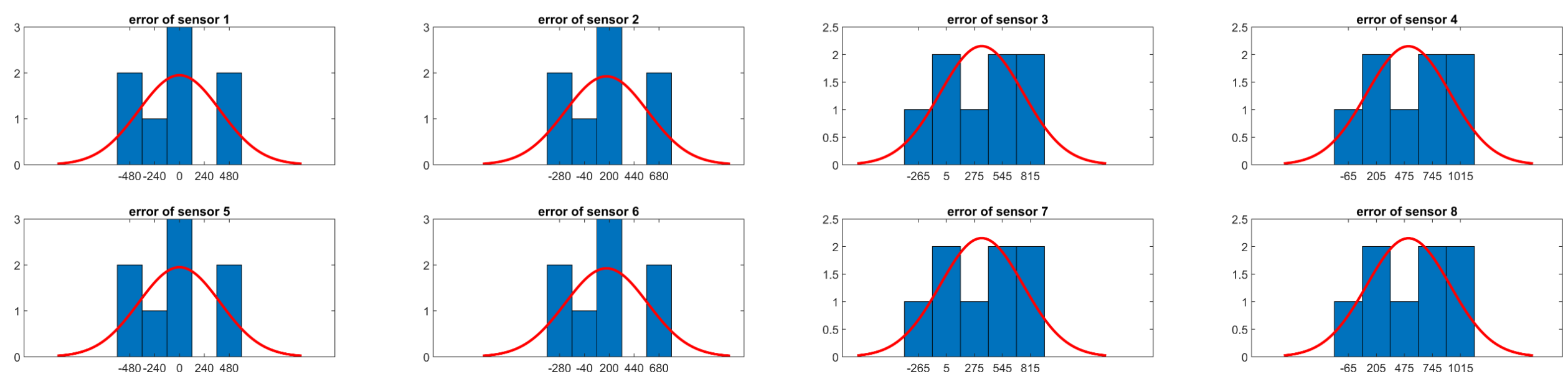
Measurement Phase

1. Setup: Randomly place the same microphones around a track.
2. Action: Collect data as the vehicle moves.

Step 2: Building Sensor Models

A time difference of arrival (TDOA) sensor network configuration knows the time of arrival of a measurement, but not the broadcast time. The TOA can be modelled as proportional to the distance (between target and sensor) plus a bias.

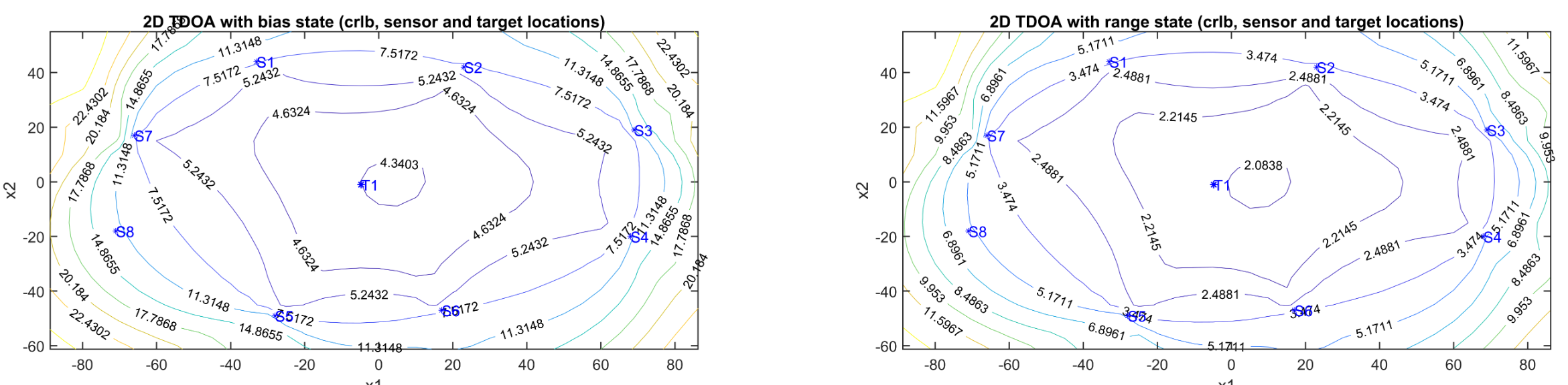
Two different 2D 8-Sensor TDOA Models will be used

1. With Bias State: Accounts for biases in the sensor network.
2. With Pairwise Differences: Focuses on time differences between sensor pairs and the vehicle.

Analyzing with Cramer-Rao Lower Bound (CRLB) can help us understand the differences between these TDOA models. The CRLB is a statistical method to estimate the lower bound of an estimator’s variance, it helps in understanding the performance and reliability of your tracking system.</li>

Step 3: Localisation and Tracking Techniques

Using Weighted Least Squares (WLS) for Localisation

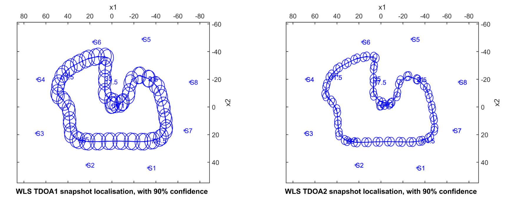
WLS is a method to minimize the differences between observed and predicted values. Here it’s used for snapshot localisation, offering a practical approach to track the vehicle’s path accurately.

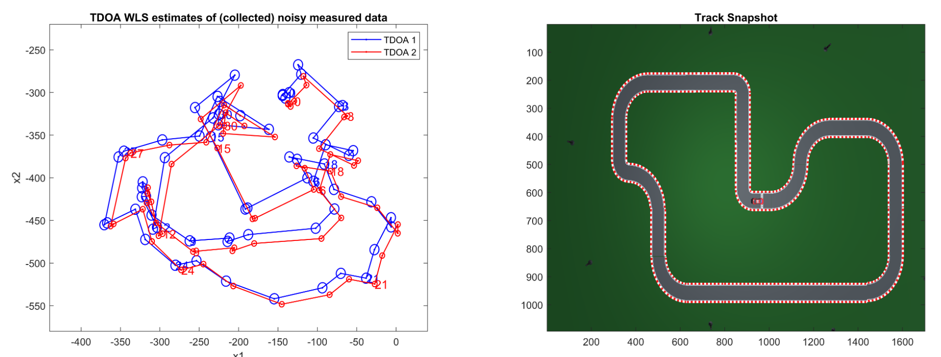
Above are the localisation results using WLS with both TDOA networks. As is evident, they are poor approximations of the track. The errors were caused by sensors skipping measurement publish intervals, only to later re-align themselves.
To fix this the data was properly aligned, the new WLS comparisons are far more faithful to the ground truth.

Implementing Extended Kalman Filter (EKF) for Localisation

The EKF combines real-time measurements with a predictive model to estimate the vehicle’s position and velocity. It’s performed in two sections, the Predictive state and the And the Update stage: The Innovation covariance is calculated, the optimal Kalman gain is computed, the Corrected estimation is updated & the Covariance is updated.

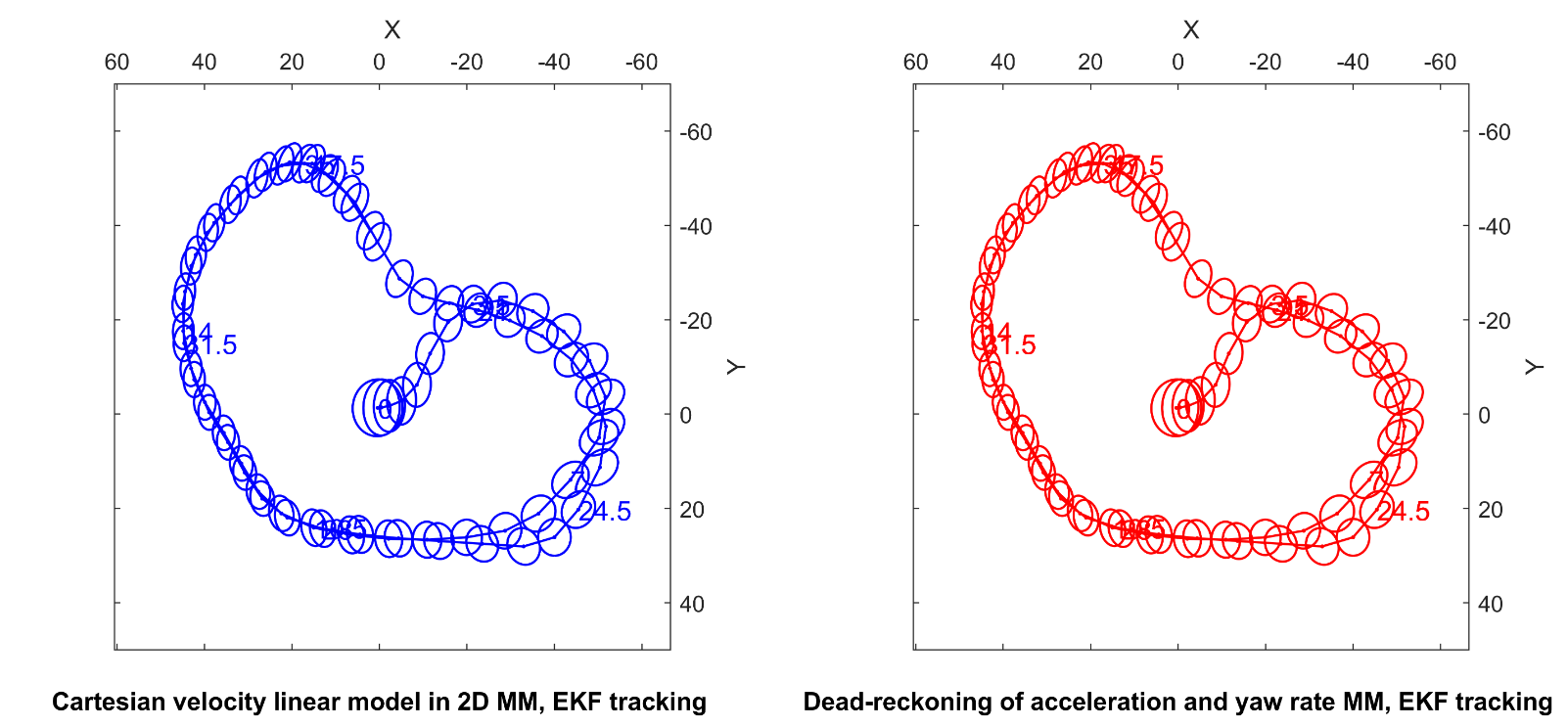
The EKF tracking here obviously underperforms compared to both the track and the WLS estimates.

Key Insights and Tips

1. Snapshot Localisation: Often more effective in scenarios where you need to track a vehicle at specific intervals.
2. Data Quality Matters: The accuracy of tracking improves with high-quality, real-world data.
3. Model Selection: The choice of sensor network and algorithms should align with your specific tracking needs.

Conclusion

Sensor fusion in vehicle localisation and tracking is a powerful technique that combines multiple data sources for enhanced accuracy. While TDOA1 & TDOA2 networks obviously differed in their variances & accuracies, the compute time for each should be considered before a best estimator can be crowned. Similarly, the WLS outperformed the EKF for this specific application, that far-from invalidates the use of the EKF. The principles and methods outlined can be applied to a multitude of different scenarios and data.

---

This post was based on my GitHub repo