In the rapidly evolving world of automotive safety, lane detection is a cornerstone technology.
It’s particularly crucial for the safe navigation of vehicles on diverse road conditions,
such as the left-hand-drive, blustery conditions of the West of Ireland.
In this project I explored a classical computer vision technique for lane detection & recognition on Sligo roads.
Methodology Unpacked
The project, developed in Python3 and employing OpenCV, is hosted on my GitHub.
It takes a unique (and perhaps not very good) approach to processing video stream data frame-by-frame,
identifying lane markings, and overlaying them onto the original video feed.
The Pre-processing Saga
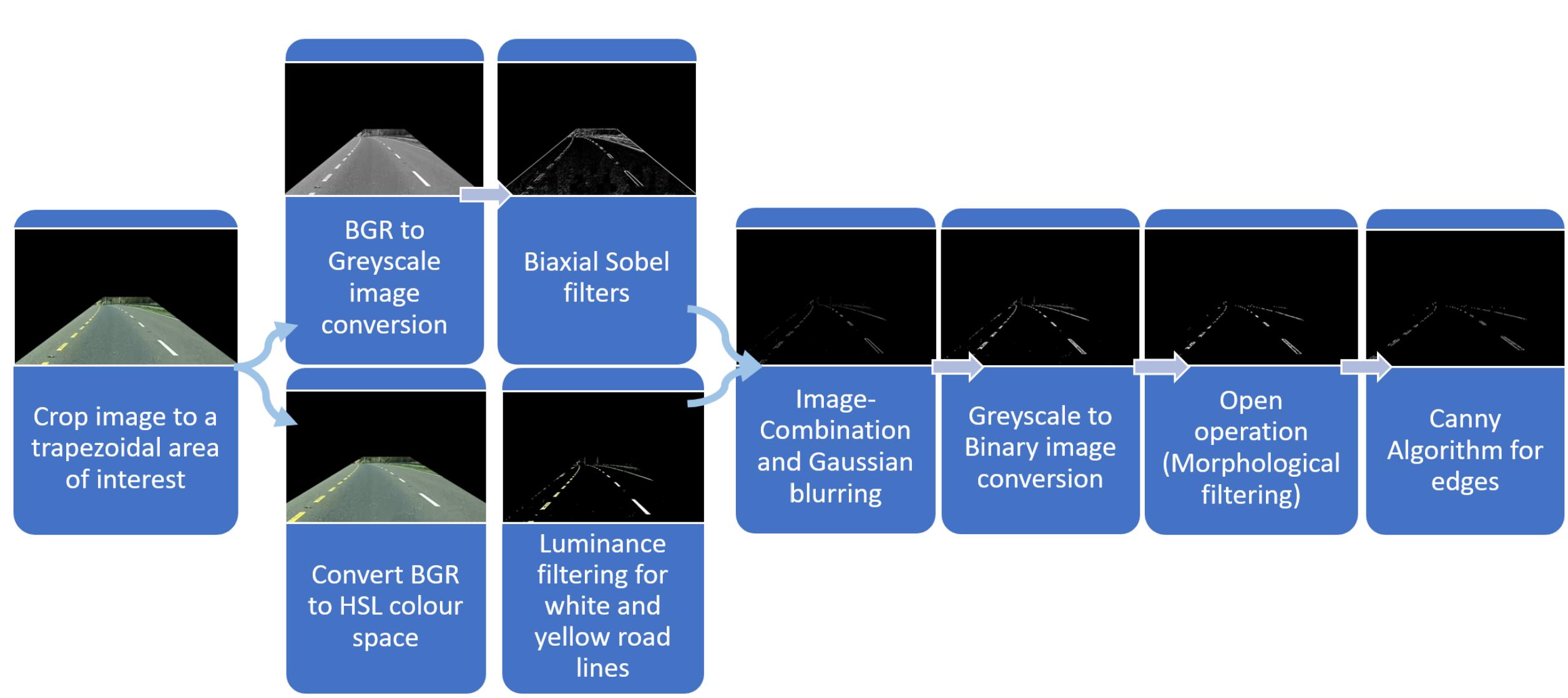
Every frame undergoes a rigorous pre-processing routine:
Area of Interest (AOI): Frames are first masked to reduce computation to the essential, road-only view.
This is achieved by defining a trapezoidal AOI based on preset coefficients.
Grayscale Conversion and Edge Detection: The image is converted to grayscale, blending the Blue-Green-Red (BGR)
channels. The Sobel–Feldman operator is then applied to highlight edges.
HSL Conversion and Thresholding: Simultaneously, the BGR image is converted to a Hue-Luminance-Saturation (HSL) representation.
The luminance is thresholded to accentuate the white or yellow lane markings, rather than tyre marks or fallen branches.
Combination: The HLS image is converted to greyscale and both images are logically ANDed together. Best of both.
Blurring, Dilating and Eroding: The combined image is blurred, converted to a binary image and a series of erosion and dilation operations are performed.
These morphological operations are effective in removing artefacts and noise remaining in the image, “opening” it.
Canny Edge Detector: Finally, the image is ready for the Canny edge detector, this will help to find lines in the image & is the last step before lane detection.
Lane Detection Mechanics
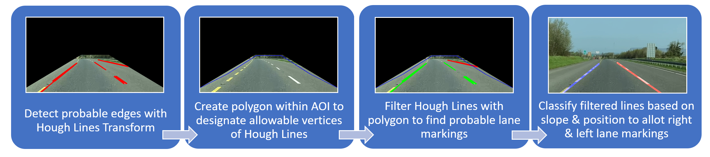
Post pre-processing, the Hough Transform algorithm comes into play..
It identifies continuous lines in the image, discerning potential lane markings based on their slopes and continuity.
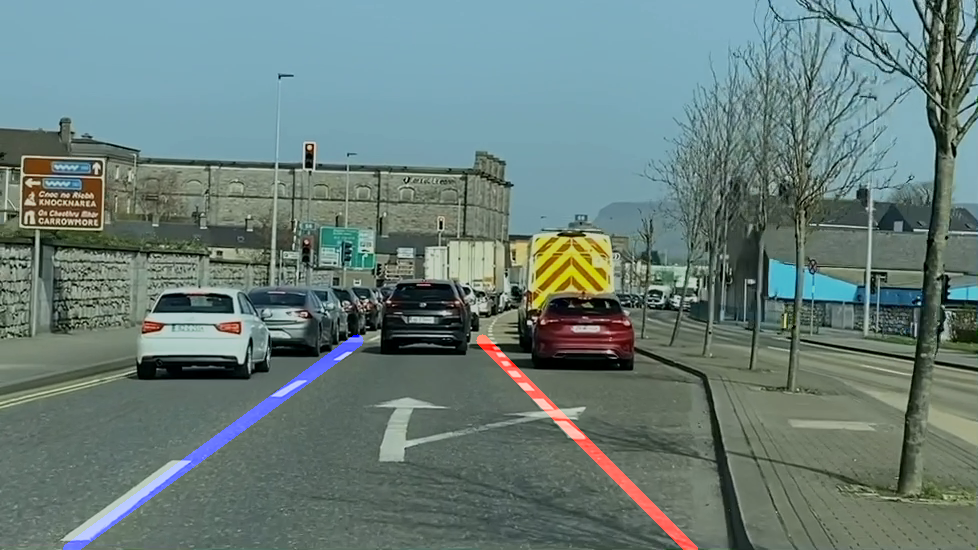
Hough lines were discarded as probable lane markings using a trapezoidal bounded filtering method.
Finally the lane lines were chosen based on the slopes and position in relation to the vehicle.
Concluding Thoughts and Beyond
This project is an example of traditional computer vision techniques in action.
The future seems to incline towards AI and deep learning models for their adaptability and dynamism, especially
under complex road conditions.
Though, it’s still relevant and helpful to understand and implement classical methods of computer vision.
There are a plethora of methods to improve this algorithm, the obvious ones to me are to:
Dynamic AOI - create an area of interest based only on the road in front.
This would help when changing lanes, pulling onto a road & allow for data from different angles/ vehicles.
Memory based lane markings - The estimation of lane markings based on expected road rules & immediately previous frame experiences.
This could be particularly useful for the many Irish roads with faded & occluded boundaries.
Other ongoing research and projects are pushing the envelope in lane detection accuracy and robustness 1.
It’s clear that the path to safe automotive transportation is both challenging and exciting, with each
new development paving the way for safer and smarter roads worldwide.
N. J. Zakaria, Et al., “Lane Detection in Autonomous Vehicles: A Systematic Review,” in IEEE Access, vol. 11, pp. 3729-3765, 2023, doi: 10.1109/ACCESS.2023.3234442. ↩
Ever fancied a drum-kit that won't take up half your living room, while still annoying your neighbours?
Well, here's a solution that might just hit the right note: an interactive, wall-projected drum-kit.
A nifty virtual kit that's a mix of clever electronics, lots of copper tape and a sprinkle of whimsy.
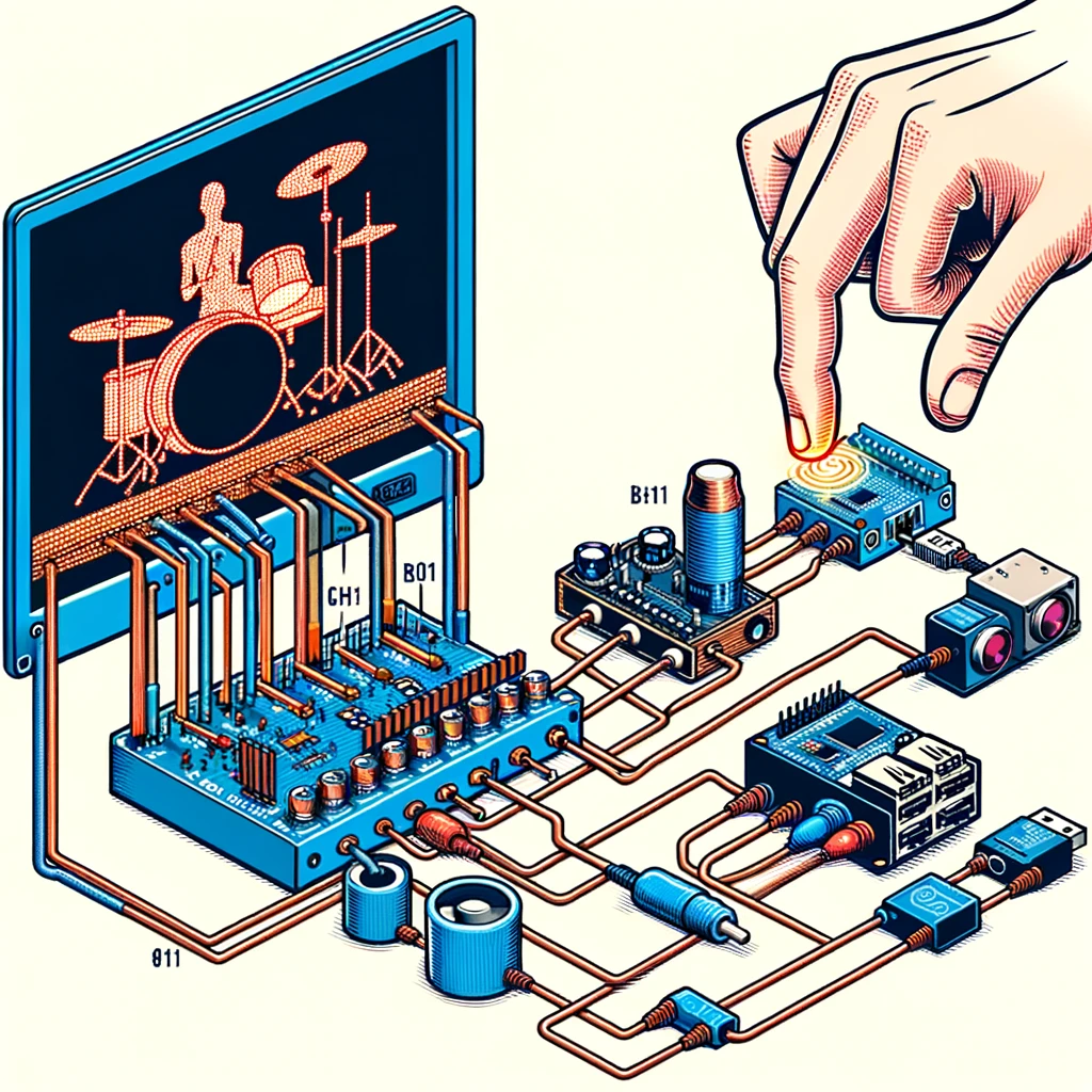
How it Works: A Symphony of Hardware and Software
The magic behind this project is a combination of Arduino and Processing sketches.
The Arduino, a master of sensing inputs, waits for a tap on the capacitive switches, via copper tape, on the wall.
Once it gets the signal, it sends the info over to the Processing sketch via serial communication.
The Arduino code is particularly simple, just sampling the capacitive switches and sending their state to Processing.
The Processing sketch is where the visual and auditory magic happens.
It creates the projected image of the drum-kit on the wall and plays the corresponding drum sounds.
And after some fiddling with wire the project is complete.
The drums are waiting.
In Conclusion: Simple, Silly, and Satisfying
The project isn’t breaking new ground in technology or art, but maybe it’s a delightful blend of both.
It’s a testament to how a simple idea, some basic coding, and a bit of hardware can lead to hours of amusement.
Whether you’re a seasoned drummer or just someone who likes hitting walls, this project hits the right notes.
A flip switch circuit for encouraging you to complete tasks, loaded with lights and achievement sounds.
This project was conceptualized and designed by me, to gamify mundane tasks. It tracks up to five tasks, offering audiovisual feedback upon completion of each task, effectively rewarding the user with a dopamine hit.
This project was more than just a tool for self-motivation; I used it as a springboard to dive into the realms of audio amplifiers and probability distributions.
Delving into the Heart of the Dopamine Box
The heart of this project lies in its Arduino code, which can be found in the Dopamine-Box.ino file.
This code is responsible for the operational logic of the box, from tracking the flip switches to triggering the lights and sounds upon task completion.
Key Interactions for the Project:
Task Tracking: Utilizes digital I/O pins to monitor the state of each flip switch.
Audio Feedback: Leverages an audio module to play sounds when a task is completed.
Visual Feedback: Controls an array of LEDs to visually indicate task progress and completion.
Haptic Feedback: Who doesn’t enjoy the satisfying snap of a throw switch.
Task Tracking:
The task completion triggers logic was as simple as it comes, the switches were polled in the main loop, waiting for an increase in the state count (number of switches flipped).
Audio Feedback:
By integrating an amplifier with the Arduino, the box produces a distinct sound each time a task is completed, amplifying the user’s sense of achievement.
I chose sounds from a variety of sources, mostly game franchises like Mario, Sonic, Legend of Zelda, etc.
I broke the 23 sounds into 5 categories, based on the expected dopamine hit.
Audio Amplification
The audio was pre-loaded onto an SD card (I fear to share it all for copyright infringement).
In my first foray into audio amplification I used an LM386 Low Voltage Power Amp and a recycled speaker I’d harvested from an old device.
Tuning the circuit was definitely the most difficult part of this project.
Trying to achieve the highest signal gain while minimising the noise was an interesting process.
Probability Distributions for Happiness Contributions
The most enjoyable part of this project was creating a state dependant probability distribution to play the 5 categories of feedback sound.
I believe the probability distribution helped to keep the task rewards unpredictable, and therefore keeping the Dopamine Box re-usable.
// Probability of output:       A,    B,    C,    X,    F},
int outputProbability[5][5] = {{80,   10,   7,    3,    0},
                               {30,   50,   15,   5,    0},
                               {5,    70,   22,   3,    0},
                               {0,    10,   85,   3,    2},
                               {0,    0,    0,    0,    100}
                              };
The columns of the above matrix represent the 5 categories of Dopamine level, while the rows represented the state count (cumulative number of switches flipped).
When a new switch is flipped, the corresponding state row is selected (eg. state = 2, outputArray = {5, 70, 22, 3, 0}).
The category probabilities are treated like a number line, where a randomised value is generated between 1-100 & the audio category chosen is based on the location of the randomised point on the number line.
Electronics
Finally, all was left was to select components, breadboard prototyping & stripboard soldering.
The Dopamine Box project was an enriching journey, blending electronics, programming, and psychological elements to create a unique, one-of-a-kind box? tool? e-waste?
At some point, I’d like to update it with a nicer chassis, perhaps an internet connection to pull hundreds of reward sounds & more enriching feedback!
All schematics, code & 3D model files can be found in the Github repo.
Within this blog we'll explore an application of sensor fusion in vehicle localisation and tracking.
It'll walk through the key concepts, methods, and reasoning behind the project.
The blog aims to provide a clear understanding of how sensor fusion works in the niche context of tracking vehicles.
Getting Started: Understanding the Basics
What is Sensor Fusion?
Sensor fusion involves combining data from multiple sensors to improve the accuracy of information.
Using multiple sensors compensates for the limitations of individual sensors, offering a more reliable and accurate tracking system.
In vehicle tracking, this means using various external/internal sensors to precisely determine a vehicle's
position and movement.
What is The Project
In this project, an eight-node sensor network will be used for vehicle tracking.
This project provides a practical example of how sensor fusion can be implemented effectively.
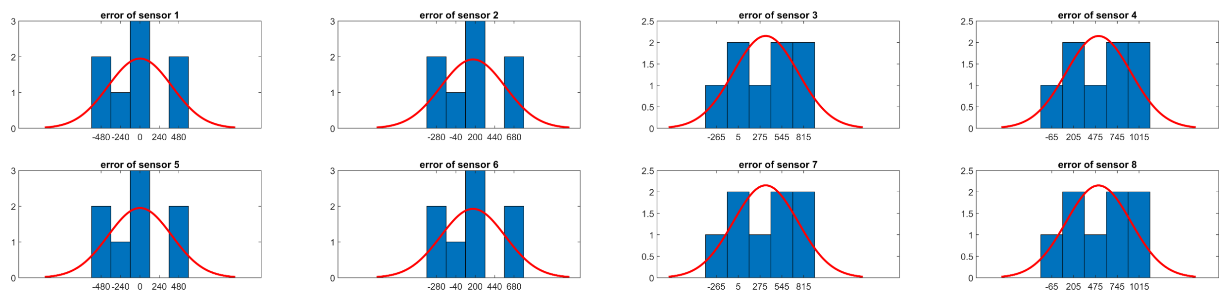
Step 1: Data Collection and Calibration
Calibration Mode
Setup: Position microphones equidistant from a stationary vehicle.
Assume the first microphone has a zero bias, all other mics are set relatively based on mic zero.
Purpose: To understand each microphone's bias, which is crucial for accurate data interpretation.
Measurement Phase
Setup: Randomly place the same microphones around a track.
Action: Collect data as the vehicle moves.
Step 2: Building Sensor Models
A time difference of arrival (TDOA) sensor network configuration knows the time of arrival of a measurement, but not the broadcast time.
The TOA can be modelled as proportional to the distance (between target and sensor) plus a bias.
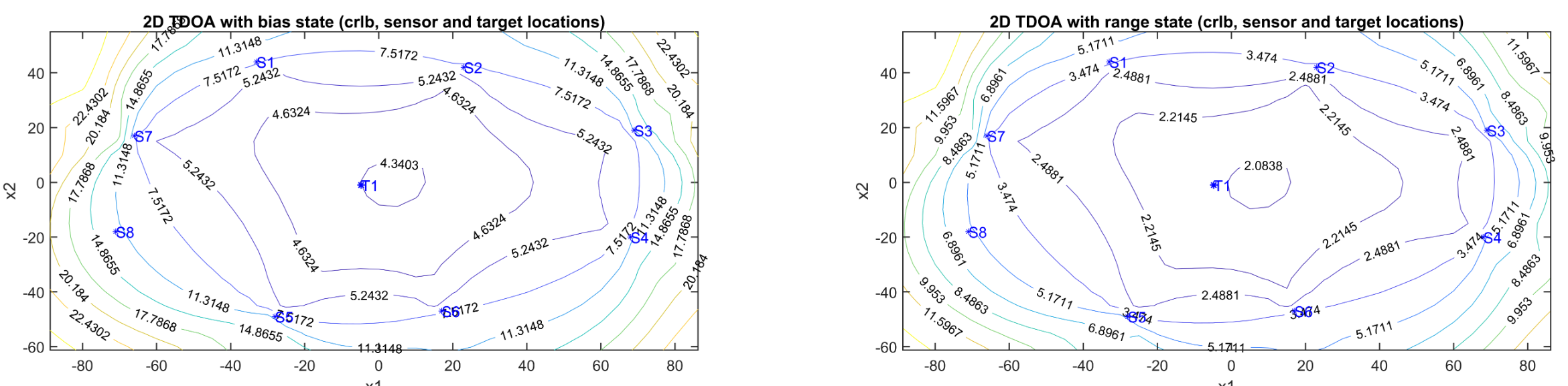
Two different 2D 8-Sensor TDOA Models will be used
With Bias State: Accounts for biases in the sensor network.
With Pairwise Differences: Focuses on time differences between sensor pairs and the vehicle.
Analyzing with Cramer-Rao Lower Bound (CRLB) can help us understand the differences between these TDOA models.
The CRLB is a statistical method to estimate the lower bound of an estimator’s variance,
it helps in understanding the performance and reliability of your tracking system.</li>
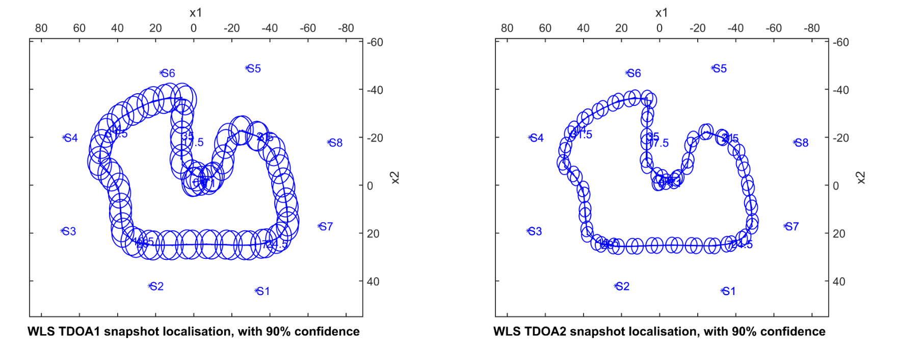
Step 3: Localisation and Tracking Techniques
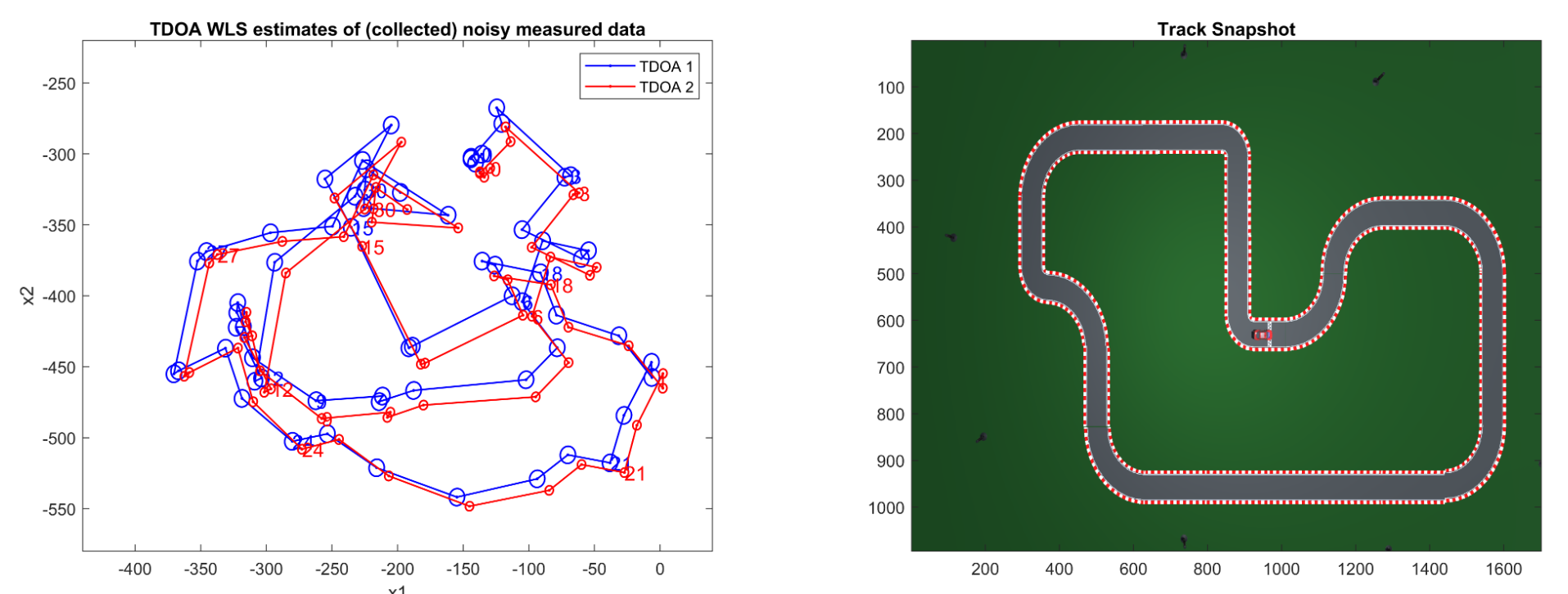
Using Weighted Least Squares (WLS) for Localisation
WLS is a method to minimize the differences between observed and predicted values.
Here it’s used for snapshot localisation, offering a practical approach to track the vehicle’s path accurately.
Above are the localisation results using WLS with both TDOA networks.
As is evident, they are poor approximations of the track.
The errors were caused by sensors skipping measurement publish intervals, only to later re-align themselves.
To fix this the data was properly aligned, the new WLS comparisons are far more faithful to the ground truth.
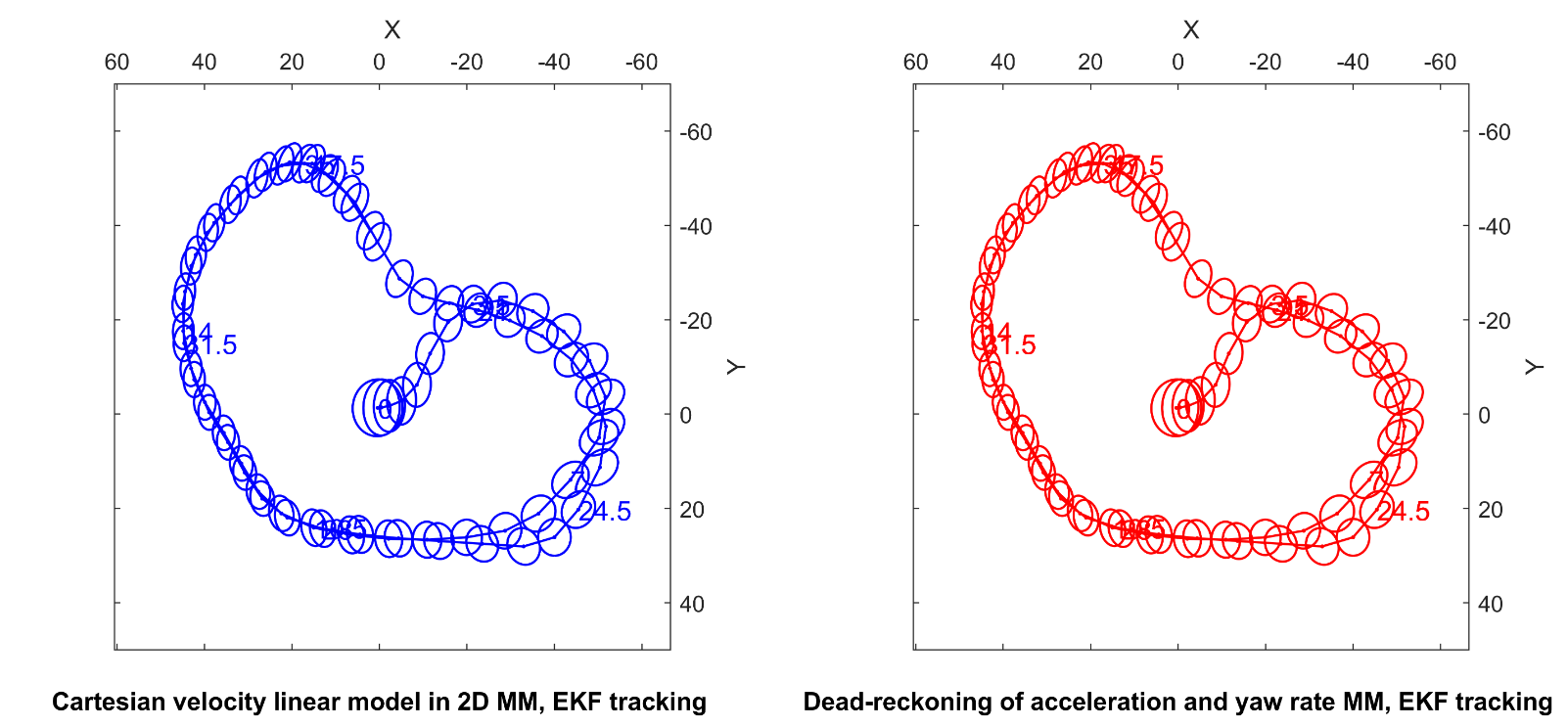
Implementing Extended Kalman Filter (EKF) for Localisation
The EKF combines real-time measurements with a predictive model to estimate the vehicle’s position and velocity.
It’s performed in two sections, the Predictive state and the And the Update stage: The Innovation covariance is calculated, the optimal Kalman gain is computed, the
Corrected estimation is updated & the Covariance is updated.
The EKF tracking here obviously underperforms compared to both the track and the WLS estimates.
Key Insights and Tips
Snapshot Localisation: Often more effective in scenarios where you need to track a vehicle at specific intervals.
Data Quality Matters: The accuracy of tracking improves with high-quality, real-world data.
Model Selection: The choice of sensor network and algorithms should align with your specific tracking needs.
Conclusion
Sensor fusion in vehicle localisation and tracking is a powerful technique that combines multiple data sources
for enhanced accuracy.
While TDOA1 & TDOA2 networks obviously differed in their variances & accuracies, the compute time for each should be considered before a best estimator can be crowned.
Similarly, the WLS outperformed the EKF for this specific application, that far-from invalidates the use of the EKF.
The principles and methods outlined can be applied to a multitude of different scenarios and data.
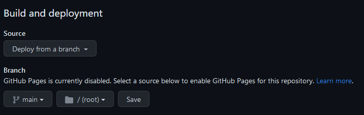
To build, host & deploy the site in the local repo directory use:
jekyll serve
In case that didn’t work properly
You may encounter some _config.yml errors using:
markdown: redcarpet
Change to markdown: kramdown
highlighter: pygments
Change to highlighter: Rouge
relative_permalinks: true
Change to relative_permalinks: false
Adding plugins: [jekyll-paginate]
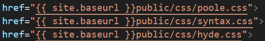
I also experienced issues with the addresses in the head.html, with the CSS links!
This was fixed by adding or removing a / before public in the URL.
Customisation
With the local copy working, you can customise the /_includes, /_layouts, /_posts, _config.yml, /public, atom.xml, 404.html, about.md & index.html pages, but not the /_site directory, as this will be overwritten with each build of the Jekyll service.
Adding Articles
Posts are added within the _posts directory, named specifically in the YYYY-MM-DD-title format.
Kramdown markdown is used to format the posts.
All written markdown articles should have some variation on the following header, called a Front Matter in Jekyll:
---layout:posttitle:How to Make a Technical Blog---
Then start writing your markdown articles and documenting your adventures.
Thanks for joining me 😊